How you can consider the LLM utilizing the embraced face analysis

Evaluation Giant language fashions (LLM) It’s important. You have to perceive how effectively they work and ensure your requirements. The Consider Face Consider library presents a helpful set of instruments for this job. This information exhibits the way to use the Consider library to guage LLM with examples of sensible code.

Perceive the embraced face analysis library

The hug face analysis library offers instruments for various analysis wants. These instruments are divided into three important classes:

1. Metrics: These measure the efficiency of a mannequin by evaluating their predictions with the labels of basic fact. The examples embrace precision, F1, Bleu and Rouge rating.
2. Comparisons: These assist examine two fashions, usually analyzing how their predictions align with one another or with reference labels.
3. Measures: These instruments examine the properties of the info units themselves, equivalent to calculating the complexity of the textual content or labeling distributions.

You’ll be able to entry all these analysis modules utilizing a single perform: Consider.load ().

Beginning

Facility

First, you should set up the library. Open your system or image of the system and execute:

pip set up consider

pip set up rouge_score # Wanted for textual content era metrics

pip set up consider(visualization) # For plotting capabilities

These instructions set up the core analysis library, the Rouge_Score package deal (required for the ROUGE Metric usually utilized in abstract), and non-obligatory dependencies for visualization, equivalent to radar graphs.

Loading of an analysis module

To make use of a selected analysis software, the load by identify. For instance, to load the precision metric:

import consider

accuracy_metric = consider.load("accuracy")

print("Accuracy metric loaded.")

Manufacturing:

This code imports the analysis and cargo library the precision metric object. Will use this object to calculate precision scores.

Primary analysis examples

Let’s stroll by means of some frequent analysis eventualities.

Pc precision instantly

You’ll be able to calculate a metric offering all references (terrestrial fact) and predictions on the identical time.

import consider

# Load the accuracy metric

accuracy_metric = consider.load("accuracy")

# Pattern floor fact and predictions

references = (0, 1, 0, 1)

predictions = (1, 0, 0, 1)

# Compute accuracy

consequence = accuracy_metric.compute(references=references, predictions=predictions)

print(f"Direct computation consequence: {consequence}")

# Instance with exact_match metric

exact_match_metric = consider.load('exact_match')

match_result = exact_match_metric.compute(references=('hey world'), predictions=('hey world'))

no_match_result = exact_match_metric.compute(references=('hey'), predictions=('hell'))

print(f"Actual match consequence (match): {match_result}")

print(f"Actual match consequence (no match): {no_match_result}")

Manufacturing:

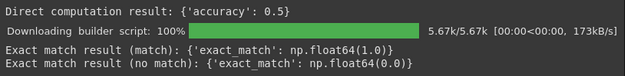
Clarification:

1. We outline two lists: the references include the proper labels and the predictions include the exits of the mannequin.
2. The calculation methodology takes these lists and calculates precision, returning the consequence as a dictionary.
3. We additionally present the exact_match metric, which verifies if the prediction coincides completely with the reference.

Incremental analysis (utilizing add_batch)

For big knowledge units, lot predictions might be extra environment friendly in reminiscence. You’ll be able to add tons incremental and calculate the ultimate rating on the finish.

import consider

# Load the accuracy metric

accuracy_metric = consider.load("accuracy")

# Pattern batches of refrences and predictions

references_batch1 = (0, 1)

predictions_batch1 = (1, 0)

references_batch2 = (0, 1)

predictions_batch2 = (0, 1)

# Add batches incrementally

accuracy_metric.add_batch(references=references_batch1, predictions=predictions_batch1)

accuracy_metric.add_batch(references=references_batch2, predictions=predictions_batch2)

# Compute closing accuracy

final_result = accuracy_metric.compute()

print(f"Incremental computation consequence: {final_result}")

Manufacturing:

Clarification:

1. We simulate processing knowledge in two tons.
2. Add_Batch updates the interior state of the metric with every lot.
3. Name Compute () with out arguments calculate the metric in all added tons.

Combining a number of metrics

Typically you wish to calculate a number of metrics concurrently (for instance, precision, F1, precision, reminiscence for classification). He Consider.mix The perform simplifies this.

import consider

# Mix a number of classification metrics

clf_metrics = consider.mix(("accuracy", "f1", "precision", "recall"))

# Pattern knowledge

predictions = (0, 1, 0)

references = (0, 1, 1) # Word: The final prediction is wrong

# Compute all metrics directly

outcomes = clf_metrics.compute(predictions=predictions, references=references)

print(f"Mixed metrics consequence: {outcomes}")

Manufacturing:

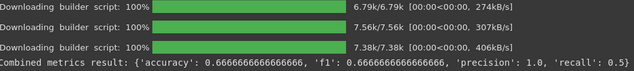
Clarification:

1. Consider.mix Take a listing of metric names and return a mixed analysis object.
2. Name pc into this object calculates all specified metrics utilizing the identical enter knowledge.

Utilizing measures

Measurements can be utilized to investigate knowledge units. Right here we present you the way to use the Word_Length measurement:

import consider

# Load the word_length measurement

# Word: Could require NLTK knowledge obtain on first run

attempt:

   word_length = consider.load("word_length", module_type="measurement")

   knowledge = ("hey world", "that is one other sentence")

   outcomes = word_length.compute(knowledge=knowledge)

   print(f"Phrase size measurement consequence: {outcomes}")

besides Exception as e:

   print(f"Couldn't run word_length measurement, presumably NLTK knowledge lacking: {e}")

   print("Trying NLTK obtain...")

   import nltk

   nltk.obtain('punkt') # Uncomment and run if wanted

Manufacturing:

Clarification:

1. We load Word_Length and specify module_type = “measurement”.
2. The computing methodology takes the info set (a sequence record right here) as an entrance.
3. Returns statistics on the lengths of the phrases within the knowledge supplied. (Word: Requires NLTK and its ‘punkt’ tokenizer knowledge).

Analysis of particular NLP duties

Completely different NLP duties require particular metrics. The embraced face analysis contains many requirements.

Automated translation (Bleu)

Bleu (bilingual analysis substitute) is frequent for the standard of translation. It measures the superposition of N-Gram between the interpretation of the mannequin (speculation) and the reference translations.

import consider

def evaluate_machine_translation(hypotheses, references):

   """Calculates BLEU rating for machine translation."""

   bleu_metric = consider.load("bleu")

   outcomes = bleu_metric.compute(predictions=hypotheses, references=references)

   # Extract the primary BLEU rating

   bleu_score = outcomes("bleu")

   return bleu_score

# Instance hypotheses (mannequin translations)

hypotheses = ("the cat sat on mat.", "the canine performed in backyard.")

# Instance references (right translations, can have a number of per speculation)

references = (("the cat sat on the mat."), ("the canine performed within the backyard."))

bleu_score = evaluate_machine_translation(hypotheses, references)

print(f"BLEU Rating: {bleu_score:.4f}") # Format for readability

Manufacturing:

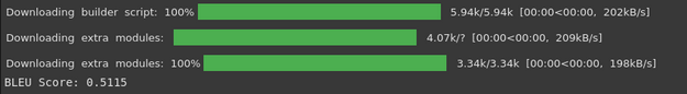
Clarification:

1. The perform masses the Metric Bleu.
2. Calculate the rating in contrast the expected translations (speculation) with a number of right references.
3. The next Blu rating (nearer to 1.0) normally signifies a greater translation high quality, which suggests extra overlap with reference translations. A rating round 0.51 suggests a average overlap.

Recognition of an entity appointed (NER – utilizing Seqeval)

For sequence labeling duties equivalent to NER, metrics equivalent to Precision, Rechinc and F1-Rating by sort of entity are helpful. Seqeval metric handles this format (for instance, b-per, i-per, or labels).

To execute the next code, the Seqeval library could be required. It might be put in by working the next command:

pip set up seqeval

Code:

import consider

# Load the seqeval metric
attempt:

   seqeval_metric = consider.load("seqeval")

   # Instance labels (utilizing IOB format)
   true_labels = (('O', 'B-PER', 'I-PER', 'O'), ('B-LOC', 'I-LOC', 'O'))

   predicted_labels = (('O', 'B-PER', 'I-PER', 'O'), ('B-LOC', 'I-LOC', 'O')) # Instance: Excellent prediction right here

   outcomes = seqeval_metric.compute(predictions=predicted_labels, references=true_labels)

   print("Seqeval Outcomes (per entity sort):")

   # Print outcomes properly

   for key, worth in outcomes.objects():

       if isinstance(worth, dict):

           print(f"  {key}: Precision={worth('precision'):.2f}, Recall={worth('recall'):.2f}, F1={worth('f1'):.2f}, Quantity={worth('quantity')}")

       else:

           print(f"  {key}: {worth:.4f}")

besides ModuleNotFoundError:

   print("Seqeval metric not put in. Run: pip set up seqeval")

Manufacturing:

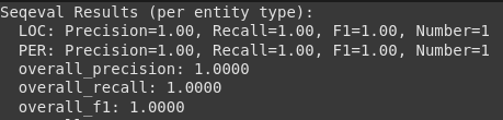
Clarification:

• We load the Seqeval metric.
• Take lists of lists, the place every inside record represents the labels for a sentence.
• The computing methodology returns the detailed precision, retirement and F1 scores for every sort of recognized entity (equivalent to PER for particular person, loc for location) and normal scores.

Textual content Abstract (Rouge)

Rouge (substitute oriented to retirement for the analysis of the connection) Examine a abstract generated with reference summaries, specializing in superimposed n-grams and the longest longer frequent.

import consider

def simple_summarizer(textual content):

   """A really fundamental summarizer - simply takes the primary sentence."""

   attempt:

       sentences = textual content.cut up(".")

       return sentences(0).strip() + "." if sentences(0).strip() else ""

   besides:

       return "" # Deal with empty or malformed textual content

# Load ROUGE metric

rouge_metric = consider.load("rouge")

# Instance textual content and reference abstract

textual content = "At the moment is an exquisite day. The solar is shining and the birds are singing. I'm going for a stroll within the park."

reference = "The climate is nice right now."

# Generate abstract utilizing the easy perform

prediction = simple_summarizer(textual content)

print(f"Generated Abstract: {prediction}")

print(f"Reference Abstract: {reference}")

# Compute ROUGE scores

rouge_results = rouge_metric.compute(predictions=(prediction), references=(reference))

print(f"ROUGE Scores: {rouge_results}")

Manufacturing:

Generated Abstract: At the moment is an exquisite day.
Reference Abstract: The climate is nice right now.
ROUGE Scores: {'rouge1': np.float64(0.4000000000000001), 'rouge2':
np.float64(0.0), 'rougeL': np.float64(0.20000000000000004), 'rougeLsum':
np.float64(0.20000000000000004)}

Clarification:

1. We load the Rouge metric.
2. We outline a simplistic abstract for demonstration.
3. The calculation calculates completely different rouge scores:
4. The scores closest to 1.0 point out a larger similarity to the reference abstract. The low scores right here replicate the essential nature of our simple_summarizer.

Query Reply (Squadron)

The squad metric is used for inquiries to reply extractive questions. Calculate the precise coincidence (EM) and the F1 rating.

import consider

# Load the SQuAD metric

squad_metric = consider.load("squad")

# Instance predictions and references format for SQuAD

predictions = ({'prediction_text': '1976', 'id': '56e10a3be3433e1400422b22'})

references = ({'solutions': {'answer_start': (97), 'textual content': ('1976')}, 'id': '56e10a3be3433e1400422b22'})

outcomes = squad_metric.compute(predictions=predictions, references=references)

print(f"SQuAD Outcomes: {outcomes}")

Manufacturing:

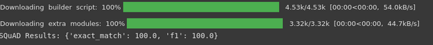
Clarification:

1. Load the squad metric.
2. Take predictions and references in a selected dictionary format, together with the expected textual content and the reality of land responses together with your beginning positions.
3. Exact_Match: Share of predictions that coincide precisely one of many responses of the reality of the soil.
4. F1: Common F1 rating on all questions, contemplating partial matches at Token degree.

Superior analysis with the analysis class

The evaluator class optimizes the method by integrating the load of the mannequin, inference and metric calculation. It’s significantly helpful for normal duties equivalent to textual content classification.

# Word: Requires transformers and datasets libraries
# pip set up transformers datasets torch # or tensorflow/jax

import consider

from consider import evaluator

from transformers import pipeline

from datasets import load_dataset

# Load a pre-trained textual content classification pipeline
# Utilizing a smaller mannequin for doubtlessly quicker execution

attempt:

   pipe = pipeline("text-classification", mannequin="distilbert-base-uncased-finetuned-sst-2-english", machine=-1) # Use CPU

besides Exception as e:

   print(f"Couldn't load pipeline: {e}")

   pipe = None

if pipe:

   # Load a small subset of the IMDB dataset

   attempt:

       knowledge = load_dataset("imdb", cut up="check").shuffle(seed=42).choose(vary(100)) # Smaller subset for pace

   besides Exception as e:

       print(f"Couldn't load dataset: {e}")

       knowledge = None

   if knowledge:

       # Load the accuracy metric

       accuracy_metric = consider.load("accuracy")

       # Create an evaluator for the duty

       task_evaluator = evaluator("text-classification")

       # Appropriate label_mapping for IMDB dataset

       label_mapping = {

           'NEGATIVE': 0,  # Map NEGATIVE to 0

           'POSITIVE': 1   # Map POSITIVE to 1

       }

       # Compute outcomes

       eval_results = task_evaluator.compute(

           model_or_pipeline=pipe,

           knowledge=knowledge,

           metric=accuracy_metric,

           input_column="textual content",  # Specify the textual content column

           label_column="label", # Specify the label column

           label_mapping=label_mapping  # Go the corrected label mapping

       )

       print("nEvaluator Outcomes:")

       print(eval_results)

       # Compute with bootstrapping for confidence intervals

       bootstrap_results = task_evaluator.compute(

           model_or_pipeline=pipe,

           knowledge=knowledge,

           metric=accuracy_metric,

           input_column="textual content",

           label_column="label",

           label_mapping=label_mapping,  # Go the corrected label mapping

           technique="bootstrap",

           n_resamples=10  # Use fewer resamples for quicker demo

       )

       print("nEvaluator Outcomes with Bootstrapping:")

       print(bootstrap_results)

Manufacturing:

Machine set to make use of cpu
Evaluator Outcomes:
{'accuracy': 0.9, 'total_time_in_seconds': 24.277618517999997,
'samples_per_second': 4.119020155368932, 'latency_in_seconds':
0.24277618517999996}
Evaluator Outcomes with Bootstrapping:
{'accuracy': {'confidence_interval': (np.float64(0.8703044820750653),
np.float64(0.9335706530476571)), 'standard_error':
np.float64(0.02412928142780514), 'rating': 0.9}, 'total_time_in_seconds':
23.871316319000016, 'samples_per_second': 4.189128017226537,
'latency_in_seconds': 0.23871316319000013}

Clarification:

1. We load a transformer pipe for textual content classification and a pattern of the IMDB knowledge set.
2. We create an evaluator particularly for “textual content classification”.
3. The calculation methodology manages the feeding knowledge (textual content column) with the pipe, acquiring predictions, evaluating them with true labels (label column) utilizing the required metric and making use of the_Mapping label.
4. Returns the metric rating along with efficiency statistics equivalent to complete time and samples per second.
5. Using technique = “Bootstrap” performs a resume to estimate belief intervals and normal error for metric, giving an thought of ​​the soundness of the rating.

Use of analysis suites

Analysis suites group a number of evaluations, usually aimed toward particular reference factors equivalent to glue. This permits a mannequin to be executed in a regular job set.

# Word: Operating a full suite might be computationally intensive and time-consuming.

# This instance demonstrates the idea however may take a very long time or require important sources.

# It additionally installs a number of datasets and should require particular mannequin configurations.

import consider

attempt:

   print("nLoading GLUE analysis suite (this may obtain datasets)...")

   # Load the GLUE job instantly

   # Utilizing "mrpc" for instance job, however you may select from the legitimate ones listed above

   job = consider.load("glue", "mrpc")  # Specify the duty like "mrpc", "sst2", and many others.

   print("Activity loaded.")

   # Now you can run the duty on a mannequin (for instance: "distilbert-base-uncased")

   # WARNING: This may take time for inference or fine-tuning.

   # outcomes = job.compute(model_or_pipeline="distilbert-base-uncased")

   # print("nEvaluation Outcomes (MRPC Activity):")

   # print(outcomes)

   print("Skipping mannequin inference for brevity on this instance.")

   print("Consult with Hugging Face documentation for full EvaluationSuite utilization.")

besides Exception as e:

   print(f"Couldn't load or run analysis suite: {e}")

Manufacturing:

Loading GLUE analysis suite (this may obtain datasets)...
Activity loaded.
Skipping mannequin inference for brevity on this instance.
Consult with Hugging Face documentation for full EvaluationSuite utilization.

Clarification:

1. Evaluationsuite.load Masses a predefined set of analysis duties (right here, solely the MRPC job from the glue reference level for the demonstration).
2. The suite command.
3. The exit is normally a listing of dictionaries, every that comprises the outcomes for a job within the suite. (Word: Executing this usually requires particular surroundings settings and substantial computing time).

Show of analysis outcomes

Visualizations assist examine a number of fashions in numerous metrics. Radar graphs are efficient for this.

import consider

import matplotlib.pyplot as plt # Guarantee matplotlib is put in

from consider.visualization import radar_plot

# Pattern knowledge for a number of fashions throughout a number of metrics

# Decrease latency is healthier, so we would invert it or take into account it individually.

knowledge = (

   {"accuracy": 0.99, "precision": 0.80, "f1": 0.95, "latency_inv": 1/33.6},

   {"accuracy": 0.98, "precision": 0.87, "f1": 0.91, "latency_inv": 1/11.2},

   {"accuracy": 0.98, "precision": 0.78, "f1": 0.88, "latency_inv": 1/87.6},

   {"accuracy": 0.88, "precision": 0.78, "f1": 0.81, "latency_inv": 1/101.6}

)

model_names = ("Mannequin A", "Mannequin B", "Mannequin C", "Mannequin D")

# Generate the radar plot

# Increased values are typically higher on a radar plot

attempt:

   # Generate radar plot (make sure you cross an accurate format and that knowledge is legitimate)

   plot = radar_plot(knowledge=knowledge, model_names=model_names)

   # Show the plot

   plt.present()  # Explicitly present the plot, may be obligatory in some environments

   # To avoid wasting the plot to a file (uncomment to make use of)

   # plot.savefig("model_comparison_radar.png")

   plt.shut() # Shut the plot window after displaying/saving

besides ImportError:

   print("Visualization requires matplotlib. Run: pip set up matplotlib")

besides Exception as e:

   print(f"Couldn't generate plot: {e}")

Manufacturing:

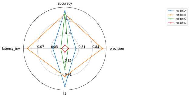
Clarification:

1. We put together pattern outcomes for 4 fashions in precision, precision, F1 and inverted latency (so it’s higher).
2. Radar_Lot creates a graph the place every axis represents a metric, which exhibits how the fashions are visually in contrast.

Save analysis outcomes

It can save you your analysis ends in a file, usually in JSON format, for report upkeep or subsequent evaluation.

import consider

from pathlib import Path

# Carry out an analysis

accuracy_metric = consider.load("accuracy")

consequence = accuracy_metric.compute(references=(0, 1, 0, 1), predictions=(1, 0, 0, 1))

print(f"Consequence to save lots of: {consequence}")

# Outline hyperparameters or different metadata

hyperparams = {"model_name": "my_custom_model", "learning_rate": 0.001}

run_details = {"experiment_id": "run_42"}

# Mix outcomes and metadata

save_data = {**consequence, **hyperparams, **run_details}

# Outline save listing and filename

save_dir = Path("./evaluation_results")

save_dir.mkdir(exist_ok=True) # Create listing if it does not exist

# Use consider.save to retailer the outcomes

attempt:

   saved_path = consider.save(save_directory=save_dir, **save_data)

   print(f"Outcomes saved to: {saved_path}")

   # It's also possible to manually save as JSON

   import json

   manual_save_path = save_dir / "manual_results.json"

   with open(manual_save_path, 'w') as f:

       json.dump(save_data, f, indent=4)

   print(f"Outcomes manually saved to: {manual_save_path}")

besides Exception as e:

    # Catch potential git-related errors if run outdoors a repo

    print(f"consider.save encountered a difficulty (presumably git associated): {e}")

    print("Trying handbook JSON save as an alternative.")

    import json

    manual_save_path = save_dir / "manual_results_fallback.json"

    with open(manual_save_path, 'w') as f:

        json.dump(save_data, f, indent=4)

    print(f"Outcomes manually saved to: {manual_save_path}")

Manufacturing:

Consequence to save lots of: {'accuracy': 0.5}
consider.save encountered a difficulty (presumably git associated): save() lacking 1
required positional argument: 'path_or_file'
Trying handbook JSON save as an alternative.
Outcomes manually saved to: evaluation_results/manual_results_fallback.json

Clarification:

1. We mix the outcomes dictionary calculated with different metadata equivalent to hyperparams.
2. Consider.Save tries to save lots of this knowledge in a JSON file within the specified listing. I might attempt to add GIT COMMIT Info in the event you run inside a repository, which might trigger errors in any other case (as seen within the authentic registry).
3. We embrace a bonus to manually save the dictionary as a JSON file, which is commonly sufficient.

Select the proper metric

Deciding on the suitable metric is essential. Take into account these factors:

1. Activity sort: Is it classification, translation, abstract, ner, qa? Use the usual of metrics for that job (precision/F1 for classification, bleu/rouge for era, seqeval for ner, squad for qa).
2. Knowledge set: Some reference factors (equivalent to glue, squad) have particular related metrics. Classification tables (for instance, in paperwork with code) usually present metric generally used for particular knowledge units.
3. Purpose: What facet of efficiency is extra necessary?
   • Accuracy: Normal correction (good for balanced courses).
   • Precision/Retirement/F1: Vital for unbalanced courses or when false positives/negatives have completely different prices.
   • Bleu/Rouge: Creep and content material overlap within the era of textual content.
   • Perplexity: How good a language mannequin predicts a pattern (decrease is healthier, it’s usually used for generative fashions).
4. Metric playing cards: Learn the metric playing cards (documentation) of hugs for detailed explanations, applicable limitations and use circumstances (for instance, Bleu card, Squad card).

Conclusion

The Consider Face Consider library presents a flexible and simple -to -use technique to consider giant language knowledge fashions and units. It offers normal metrics, measurements of the info set and instruments equivalent to Evaluator and Evaluationsuite To optimize the method. Through the use of these instruments and selecting applicable metrics on your job, you may get hold of clear details about the strengths and weaknesses of your mannequin.

For extra particulars and superior use, see official sources:

Harsh Mishra is an IA/ml engineer who spends extra time speaking with giant language fashions than actual people. Enthusiastic about Genai, NLP, and make smarter machines (in order that they nonetheless don’t change it). When it doesn’t optimize the fashions, it’s in all probability optimizing its espresso consumption.